Efficient Learning of High Level Plans from Play
Abstract
Real-world robotic manipulation tasks remain an elusive challenge, since they involve both fine-grained environment interaction, as well as the ability to plan for long-horizon goals. Although deep reinforcement learning (RL) methods have shown encouraging results when planning end-to-end in high-dimensional environments, they remain fundamentally limited by poor sample efficiency due to inefficient exploration, and by the complexity of credit assignment over long horizons. In this work, we present Efficient Learning of High-Level Plans from Play (ELF-P), a framework for robotic learning that bridges motion planning and deep RL to achieve long-horizon complex manipulation tasks. We leverage task-agnostic play data to learn a discrete behavioral prior over object-centric primitives, modeling their feasibility given the current context. We then design a high-level goal-conditioned policy which (1) uses primitives as building blocks to scaffold complex long-horizon tasks and (2) leverages the behavioral prior to accelerate learning. We demonstrate that ELF-P has significantly better sample efficiency than relevant baselines over multiple realistic manipulation tasks and learns policies that can be easily transferred to physical hardware.
Video
A.1 Environment
A.1.1 Training environment
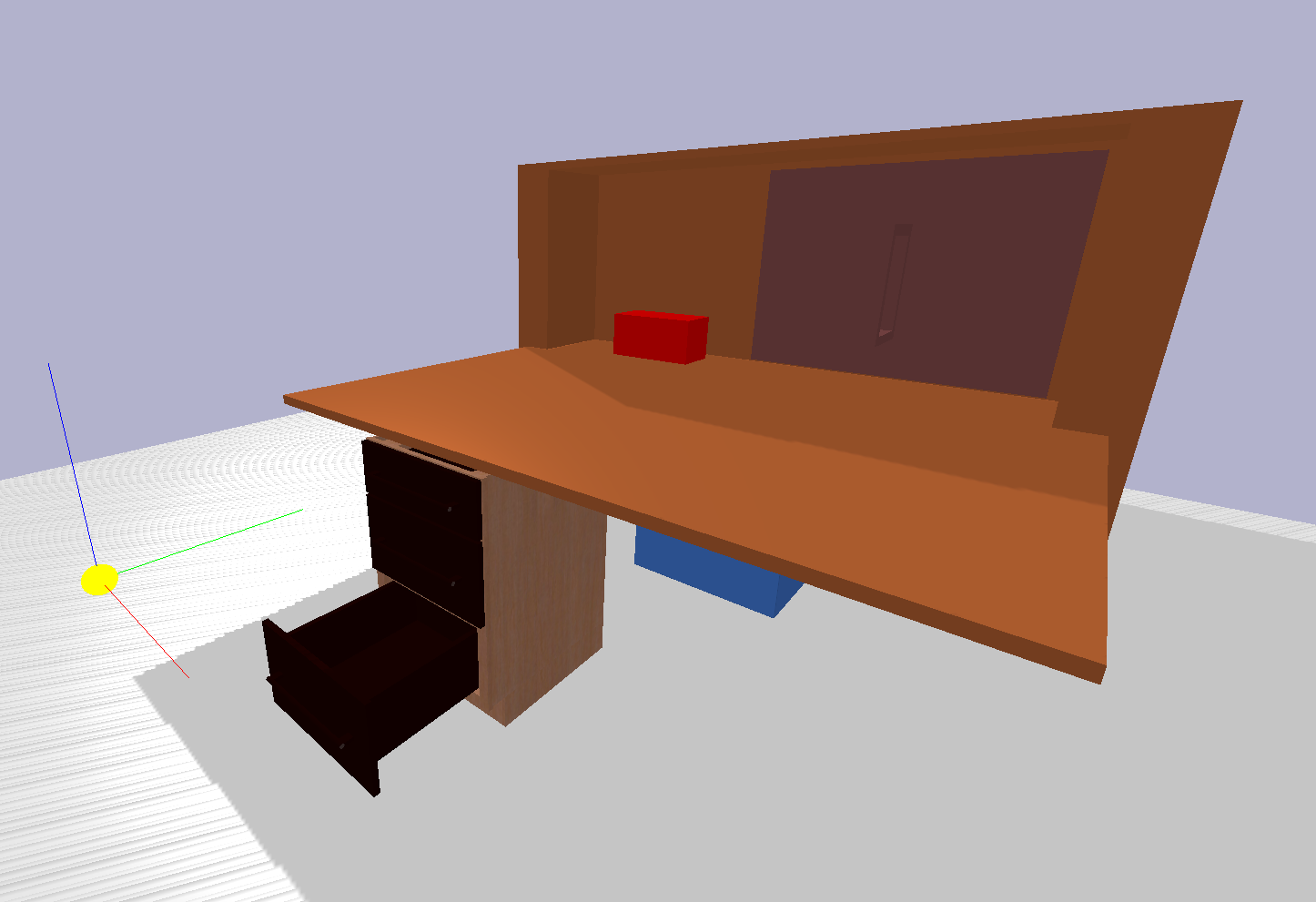
The environment is built on Pybullet physics simulation software [14] and it is shown in Figure S1. The states \(\in \mathbb{R}^{11}\) include the 3D robot's end-effector position, a binary variable representing the gripper state (open/close), the 3D position of the block and the 1D joint position for each of the 3 drawers and the door. The goal state \(\in \mathbb{R}^3\) is the desired block position (e.g. behind the door, inside the mid-drawer or somewhere on the table). The action space is discrete and consists of 10 object-centric motion primitives, namely reaching every object, manipulating the objects (e.g. sliding or pulling), and opening and closing the gripper. Given the primitives we use are relational to objects they become implicitly parameterized by the corresponding object pose. We also include a center action to move the robot back to the center of the desk to have greater reachability. Finally, we also include a go-to-goal primitive that moves the end-effector over the goal position. A complete action list is shown below:
Go to door handle
Go to drawer1 handle
Go to drawer2 handle
Go to drawer3 handle
Go to center
Go to block
Go to goal
Grasp/release (Open/close the gripper)
Pull/push
Slide left/slide right
In the case of multiple primitives for one action (i.e. actions 8, 9 and 10), the executed primitive depends on the current state (e.g. the gripper opens if its current state is closed and viceversa).
If the agent attempts an infeasible action, such as manipulating an object with the wrong primitive (e.g. pulling a sliding door) or moving in a non collision-free path, the environment does not perform a simulation step and the state remains unaltered. To check for collisions, we use the method in Pybullet, which performs a single raycast.
We use the sparse reward signal: \(R(\cdot|s, g) = 𝟙_{\{|f(s)-g|_1 < \epsilon\}}\), where \(f(s)\) extracts the current block position from the state and \(\epsilon=0.1\) is a threshold determining task success.
A.2 Extended Experimental Results
A.2.1 HER
We experiment with combining our method with off-policy goal relabeling [34]. We evaluate different relabeling ratios \(k\). As already mentioned in the Results, we observe that the greater the relabeling ratio, the slower the convergence to the optimal policy (see Figure S2). We hypothesize that this is because the environment dynamics are not smooth and the policy fails to generalize to distant goals despite the relabeling, which may hurt performance.

A.2.2 Sample complexity
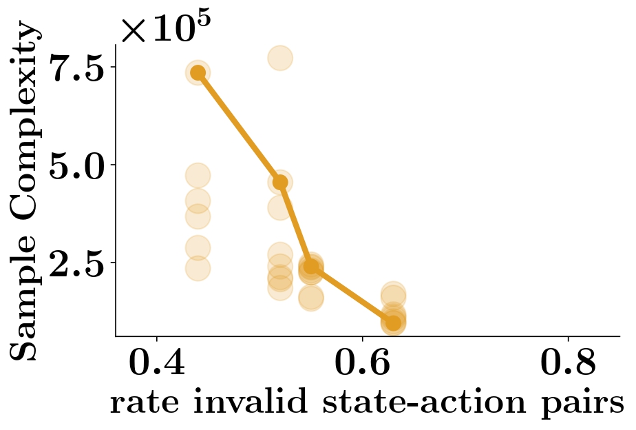
Results reported in Subsection V-A3) Sample Complexity (main paper) are obtained by running 5 independent random seeds for each value of \(\rho\) in the Medium task. We report results obtained for the Hard task in Figure S3, which shows an increase of sample complexity as the number of feasible actions increases. However, in this hard setting, several seeds for several values of \(\rho\) don’t reach a success rate of 0.95. This is expected given that for example \(\rho=0\) recovers DDQN behavior which was shown to fail in learning the Hard task. Consequently, in order not to bias the results, we opt for only reporting the results on \(\rho\) values whose seeds are always successful in learning.
A.2.3 Robustness to play dataset size
We study the effect of play dataset size on training performance for
both ELF-P and DDQN+Prefill (which affects the amount of data used for
training the prior for ELF-P and the amount of data used to prefill the replay
buffer for DDQN+Prefill). In Figure S4
we show the resulting training curves using 3 different dataset sizes
for ELF-P and DDQN+Prefill.

A.2.4 Robustness to imperfect skill execution
In this experiment, we evaluate how robust the trained agent is to imperfect skill execution. We perform test-time evaluations in which we simulate that the execution of the slide, pull/push and grasp skills is not successful with some probability. We specifically simulate that the execution of slide (pull/push) skill fails by setting the door (drawer) joint positions to random configurations whereas we simulate that the execution of grasp skill is unsuccessful by not updating the grasp state. In Table S1, we report average success rate with increasing failure probabilities for ELF-P and the most competitive baseline DDQN+Prefill on the Hard task. We observe that despite training with perfect skill execution, ELF-P is relatively robust to imperfect skill execution and it is able to generalize to out of training distribution states, whereas DDQN+Prefill is less robust to skill execution failure.
| Skill failure probability | Success rate ELF-P | Success rate DDQN+Prefill | ||||
|---|---|---|---|---|---|---|
| 0 | 1.0 \(\pm\) 0.00 | 1.0 \(\pm\) 0.00 | ||||
| 0.05 | 0.99 \(\pm\) 0.01 | 0.96 \(\pm\) 0.01 | ||||
| 0.1 | 0.96 \(\pm\) 0.02 | 0.92 \(\pm\) 0.00 | ||||
| 0.2 | 0.91 \(\pm\) 0.02 | 0.84 \(\pm\) 0.03 | ||||
| 0.5 | 0.75 \(\pm\) 0.03 | 0.54 \(\pm\) 0.04 |
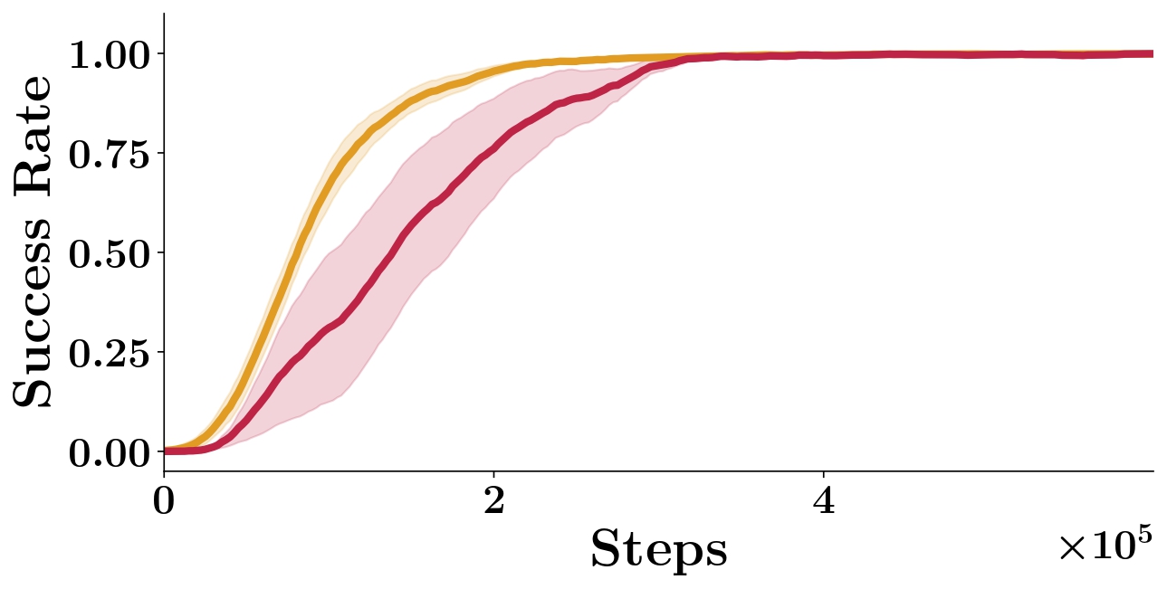
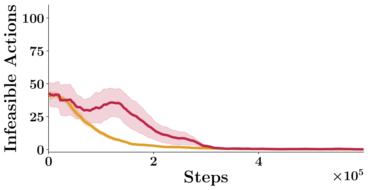
A.2.5 Soft prior integration
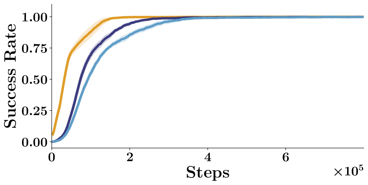
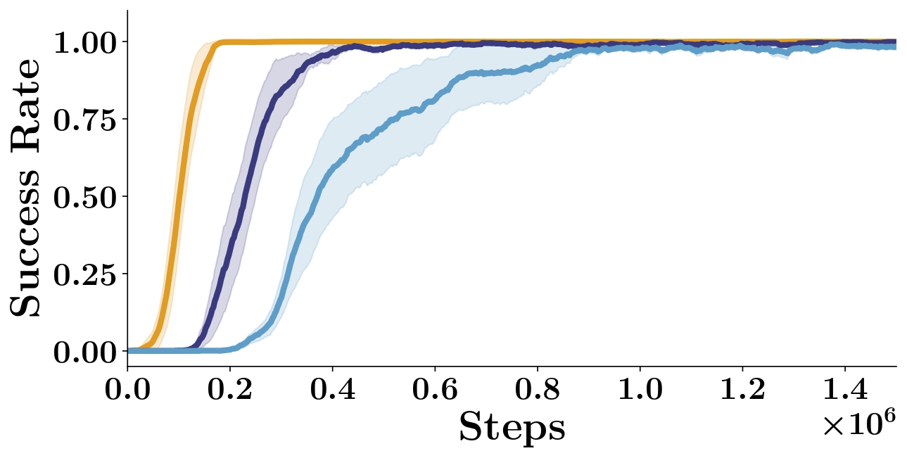
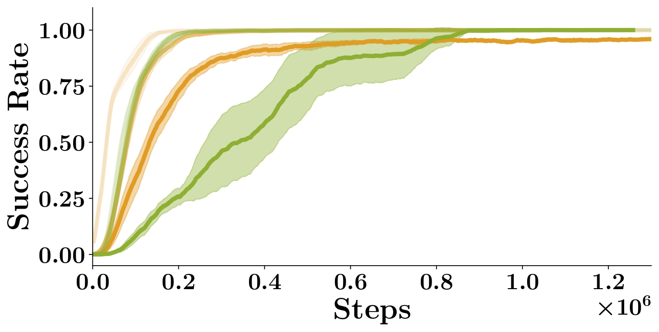
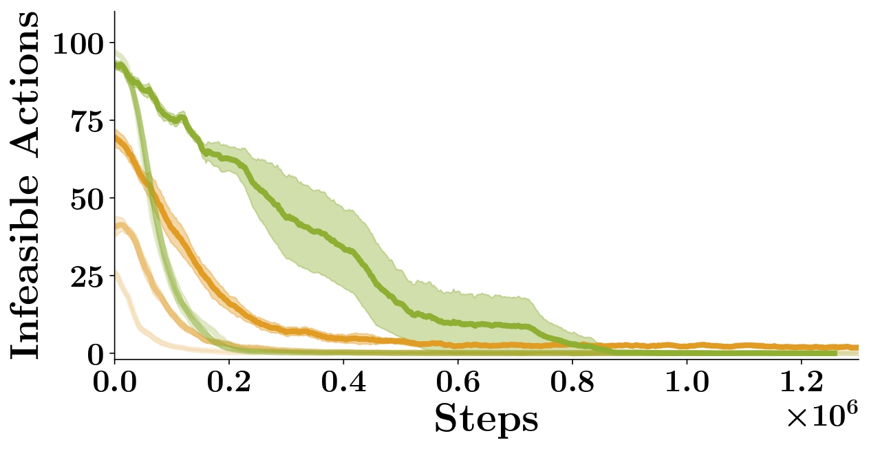
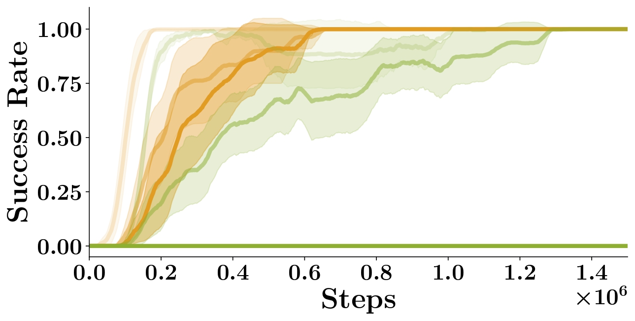
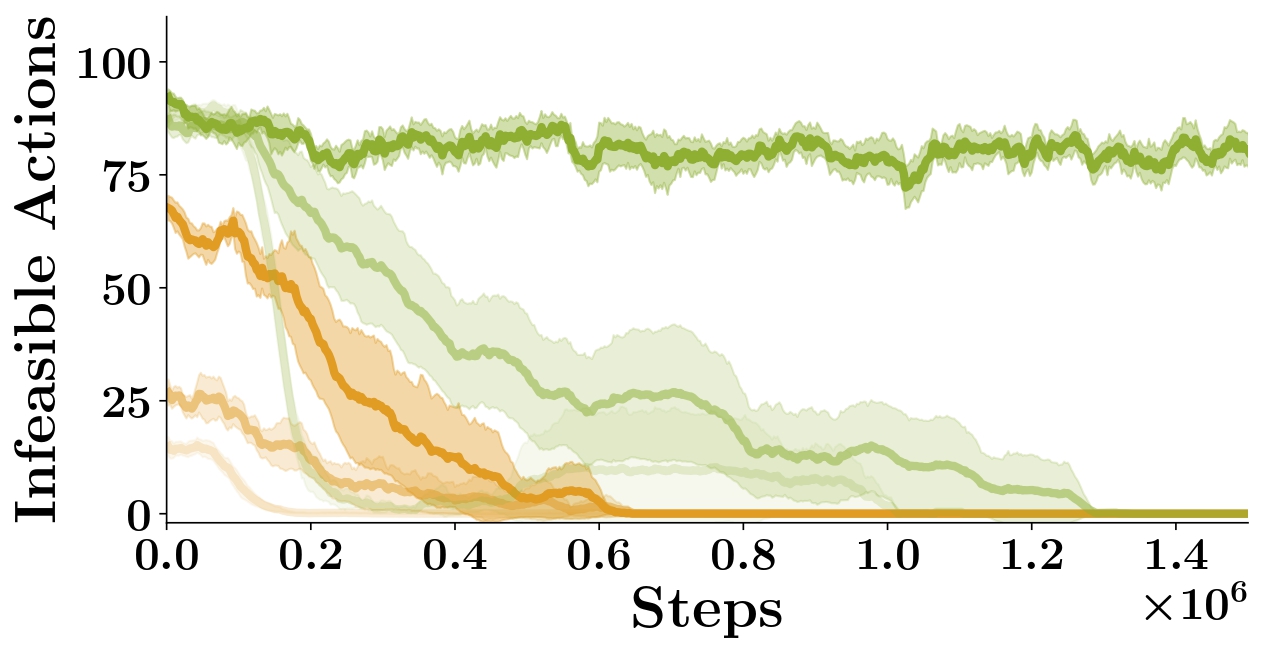
We report results on the (M) task for the Soft prior integration experiment (see Subsection V.A.3 in main paper). In Figure [fig:soft_vs_hard] we compare the performance of ELF-P with Soft-ELF-P. We observe that while Soft-ELF-P is able to learn both medium and hard tasks, it has lower sample efficiency than ELF-P. One of the main reasons of ELF-P being faster is because a hard prior integration alleviates the Q-network from learning values for all state-action pairs: it can focus on learning Q-values for feasible state-action pairs only and ignore Q-values for unfeasible actions. This shows one of the main contributions of our algorithm. Nevertheless, a soft integration could be useful when dealing with degenerated priors and we reserve further exploration on the topic for future work.

 id="fig:soft_vs_hard_appendix"/>
A.3 Additional experimental details
A.3.1 Evaluation protocol
All reported results are obtained by evaluating the policies over 50 episodes every 2500 environment steps. Results are averaged over 10 random independent seeds unless explicitly stated. Shaded areas represent standard deviation across seeds.
A.3.2 Play-dataset collection
Given that our method can learn with very little data (\(\sim\)1h30min of data collection), play data could in practice be collected by a few human operators choosing from a predefined set of primitives. However for simplicity, we resort to evaluating whether a termination condition for each primitive is met in every configuration. This is a common approach under the options framework [30]. The tuples \((s,a)\), containing the state of the environment and the feasible action performed in the state respectively, are stored in the play-dataset \(\mathcal{D}\) for training the prior.
A.3.3 Hyperparameters and Architectures
Across all baselines and experiments, unless explicitly stated, we use the same set of hyperparameters and neural network architectures Values are reported in Table Table S2. We choose a set of values that was found to perform well in previous works. We report the list of hyperparameters that were tuned for each method in the following subsections.
| Parameter | Value | |
|---|---|---|
| Q-network architecture | MLP \( [128, 256]\) | |
| Batch size | \(256\) | |
| Exploration technique | \(\epsilon\)-greedy with exponential decay | |
| Initial \(\epsilon\) | \(0.5\) | |
| Decay rate for \(\epsilon\) | \(5e^{-5}\) | |
| Discount \(\gamma\) | \(0.97\) | |
| Optimizer | Adam (\(\beta_1=0.9, \beta_2=0.999\)) [15] | |
| Learning rate \(\eta\) | 1e-4 | |
| Episode length \(T\) | \(100\) | |
| Experience replay size | \(1e^{6}\) | |
| Initial exploration steps | \(2000\) | |
| Steps before training starts | \(1000\) | |
| Steps between parameter updates | \(50\) | |
| Soft target update parameter \(\mu\) | \(0.995\) | |
| Threshold \(\rho\) | \(0.01\) |
| Parameter | Value | |
|---|---|---|
| Prior architecture | MLP \([200,200]\) | |
| Prior batch size | \(500\) | |
| Prior training steps | \(1e^{-5}\) | |
| Dataset size | \(10000\) | |
| Prior optimizer | Adam(\(\beta_1=0.9, \beta_2=0.999\) [15] | |
| Learning rate | \(1e^{-3}\) |
Discount \(\gamma\): \(0.97\). Tuned over \([0.90, 0.95, 0.97, 0.99]\).
Relabeling ratio \(k\): \(4\) (as suggested in the original paper [34]).
Discount \(\gamma\): \(0.97\). Tuned over \([0.90, 0.95, 0.97, 0.99]\).
Discount \(\gamma\): \(0.95\). Tuned over \([0.90, 0.95, 0.97, 0.99]\).
Prefill dataset: The dataset used to prefill the replay buffer is the same as the Play-dataset used to train the behavioral prior, but extending the tuples \((s,a) \to (s,a,s',g,r)\) to be able to perform TD-loss on them. Given that the Play-dataset is task-agnostic, we decide to compute the rewards with relabelling, i.e., to relabel the \(g\) to the achieved goal and to sgoal et the reward \(r\) to \(1\), otherwise set the reward to zero. We experiment with different relabeling frequencies \(f \in [0.0, 0.25, 0.5, 0.75, 1.0]\). We find that \(f>0\) leads to overestimation of the Q-values at early stages of training and thus hurt performance. For this reason we use \(f=0\), i.e., no relabelling.
Discount \(\gamma\): \(0.95\). Tuned over \([0.90, 0.95, 0.97, 0.99]\).
Large margin classification loss weight \(\lambda_2\): \(1e^{-3}\). Tuned over \([1e^{-2}, 1e^{-3}, 1e^{-4}, 1e^{-5}]\).
Expert margin: \(0.05\). Tuned over \([0.01, 0.05, 0.1, 0.5, 0.8]\).
L2 regularization loss weight \(\lambda_3\): \(1e^{-5}\).
Prefill dataset: Same approach as for DDQN+Prefill explained above.
Discount \(\gamma\): \(0.97\). Tuned over \([0.90, 0.95, 0.97, 0.99]\).
Discount \(\gamma\): \(0.97\). Tuned over \([0.90, 0.95, 0.97, 0.99]\).
KL weight \(\alpha\): \(0.01\) Tuned over \([0.005, 0.01, 0.05]\).
Actor-network architecture: MLP \( [128, 256]\)
Discount \(\gamma\): \(0.97\). Tuned over \([0.90, 0.95, 0.97, 0.99]\).
Prior training: we use the parameters reported in Table S3.
A.4 Hardware experiments
The experiments are carried out on a real desktop setting depicted in Figure 1 (main paper)(upper right). We use Boston Dynamics Spot robot [56] for all our experiments. The high-level planner, trained in simulation, is used at inference time to predict the required sequence of motion primitives to achieve a desired goal. The motion primitives are executed using established motion planning methods [73] to create optimal control trajectories. We then send desired commands to Spot using Boston Dynamics Spot SDK, a Python API provided by Boston Dynamics, which we interface with using pybind11. We refer the reader to the Video material for a visualization of the real-word experiments.
A.5 Optimality
Let us consider an MDP \(\mathcal{M}\), the reduced MDP \(\mathcal{M'}\) as defined in Subsection IV-C) Learning in a Reduced MDP (main paper), the selection operator \({\alpha: \mathcal{S \to P(A)}}\) and a set of feasible policies under \(\alpha\): \(\Pi_\alpha=\{ \pi | \pi(s,g) \in \alpha(s) \forall s \in \mathcal{S}, g \in \mathcal{G} \}\).
Given an MDP \(\mathcal{M}\), the reduced MDP \(\mathcal{M'}\) and a selection operator \(\alpha\) such that the optimal policy for \(\mathcal{M}\) belongs to \(\Pi_\alpha\) (that is \(\pi_{\mathcal{M}}^*(s, g) \in \Pi_\alpha\)), the optimal policy in \(\mathcal{M'}\) is also optimal for \(\mathcal{M}\), i.e. \(\pi_{\mathcal{M'}}^*(s, g) = \pi_{\mathcal{M}}^*(s, g)\).
Proof. We can define a goal-conditioned value function \(V^\pi(s,g)\), defined as the expected sum of discounted future rewards if the agent starts in \(s\) and follows policy \(\pi\) thereafter: \({V^\pi(s, g) = \mathbb{E}_{\mu^\pi}\left[\sum_{t-1}^\infty \gamma^{t-1} R(s, g) \right]}\) under the trajectory distribution \({\mu^\pi(\tau|g) = \rho_0(s_0) \prod_{t=0}^\infty P(s_{t+1}|s_t, a_t)}\) with \(a_t = \pi(s_t, g) \; \forall t\). By construction, the transition kernel \(P\) and the reward function \(R\) are shared across \(\mathcal{M}\) and \(\mathcal{M'}\), and a feasible policy \(\pi\) always selects the same action in both MDPs, thus trajectory distributions and value functions are also identical for feasible policies. More formally, if \(\pi \in \Pi_\alpha\), then \(\mu^\pi_{\mathcal{M}}=\mu^\pi_{\mathcal{M'}}\) and \(V^\pi_{\mathcal{M}}(s, g) = V^\pi_{\mathcal{M'}}(s, g)\).
It is then sufficient to note that \[\pi_{\mathcal{M'}}^*(s, g)\stackrel{def}{=}\arg\max_{\pi \in \Pi_\alpha} V^{\pi}_{\mathcal{M'}}(s, g)=\arg\max_{\pi \in \Pi_\alpha} V^{\pi}_{\mathcal{M}}(s,g)=\arg\max_{\pi \in \Pi} V^{\pi}_{\mathcal{M}}(s, g)\stackrel{def}{=}\pi_{\mathcal{M}}^*(s, g),\] where the second equality is due to the previous statement, and the third equality is granted by the assumption that the optimal policy for \(\mathcal{M}\) is feasible in \(\mathcal{M'}\) (i.e. \(\pi_\mathcal{M}^* \in \Pi_\alpha\)).◻
Hence, our proposed algorithm, which allows us learning directly on the reduced MDP \(\mathcal{M'}\), can under mild assumptions retrieve the optimal policy in the original \(\mathcal{M}\).
We finally remark that model-free PAC-MDP algorithms have shown to produce upper bounds on sample complexity that are \(\tilde O(N)\), where \(N \leq |\mathcal{S}||\mathcal{A}|\)[64], i.e., directly dependent on the number of state-action pairs. Hence, learning in the reduced MDP \(\mathcal{M'}\) instead of \(\mathcal{M}\) could lead to near-linear improvements in sample efficiency as the number of infeasible actions grows. We demonstrate it empirically in the Subsection V-A3) Sample Complexity (main paper) and A.2.2 Sample Complexity .